This summer I spend my time in Ecole Centrale Paris, trying to run a computer simulation on NPLIN.I will post about that later, but this was my first introduction to molecular dynamics simulation, and there I faced many problems.So I thought to write up a bit, in case it might be of help for someone in future.I am posting this , but you sure can find help from the DISCO forums.And yes, read through the manual!!
In this, I explain how we can run DL_POLY in parallel.It really did a 30 minuite simulation in 30 seconds in my 4X2 core processor in laptop
Installation:
1.Download DL_POLY_4 from ftp://ftp.dl.ac.uk/ccp5/DL_POLY/
2.Obtain Liscense by mailing the authors for home/personal/educational use
3.Unzip,Untar,Unencrypt
4.In Linux install open mpi by typing
$ sudo apt-get install libopenmpi-dev openmpi-bin openmpi-doc
$ sudo apt-get install ssh
Generate keys and add to ssh
$ ssh-keygen -t dsa
$ cat id_dsa.pub >> authorized_keys
Test program:
#include <stdio.h>
#include <mpi.h>
int main(int argc, char** argv)
{
int myrank, nprocs;
MPI_Init(&argc, &argv);
MPI_Comm_size(MPI_COMM_WORLD, &nprocs);
MPI_Comm_rank(MPI_COMM_WORLD, &myrank);
for (;;){
printf(“Hello from processor %d of %d\n”, myrank, nprocs);
}
MPI_Finalize();
return 0;
}
Testing:
$ mpicc MPI_Hello.c -o MPI_Hello
$ mpiexec -n 5 MPI_Hello #specify to run on 5 processors,press Ctrl+Z to exit
You can install htop to see if the process is really parallel [sudo apt-get install htop]
Compiling DL_POLY for Laptop Dell XPS 15z
Requires fortran to be installed.[sudo apt-get install gfortran]
1.In the DL_POLY directory>Build>copy “Makefile_MPI” to source directory and rename to “make”
2.In terminal type “sudo make hpc”
3.The process will create a DLPOLY.Z in the execute directory. Which also has a JAVA gui which can be used.(Personally I find using GUI a bit cumbersome and problematic,so I run using terminal)
4. Terminal >browse to DL_POLY execcute directory> type $./gui to invoke gui
Running sample scripts:
Some example and basic examples can be found online in
http://www.ccp5.ac.uk/DL_POLY/TUTORIAL/EXERCISES/
Although they used GUI, I am going to use a mixture of both
DLPOLY requires some necessary files to run a simulation,The CONTROL,CONFIG,FIELD files.I am going to explain them as we go,but first lets see if its working!
Download the files for EXERCISE 1 which finds out the phase transition for KCl.
The CONFIG file lists the system in brief,it gives the coordinates and velocities of all atoms in the system in initial condition.
The CONTROL file is important,it determins the thermodynamics of the system.The temperature, pressure, cutoff, and configuration like NVT,NPT etc.
FIELD defines any other field which cannot be characterised by concrete mathematical formulas
The CONFIG file uses its own self-consistent set of units.
| physical quantity | symbol | unit value |
| time | t0 | 1×10⁻¹² seconds (picoseconds) |
| length | l0 | 1×10⁻¹⁰ metres (Angstroms) |
| mass | m0 | 1.66054×10⁻²⁷ kilograms (amu) |
| charge | q0 | 1.60218×10⁻¹⁹ Coulombs (electron charge) |
| energy | E0=m0(l0/t0)2 | 1.66054×10⁻²³ Joules = 10 J mol−1 |
| pressure | p0=E0/l30 | 1.66054×10⁷ Pascal = 166.054 bar |
| Planck constant | ℏ | 6.35078E0t0 |
| Boltzmann constant | kB | 0.83145E0/K |
The others can be found from the user manual(Page 7 of DL_POLY_4_USER_MANUAL)
will learn the process through a process through the first example of DL_POLY guide.i.e. phase transition of KCl
http://www.ccp5.ac.uk/DL_POLY/TUTORIAL/EXERCISES/expmt1.html
This exercise studies a well-known phase transition in potassium chloride using constant pressure molecular dynamics. The objective is to develop the best practice in using such algorithms and to learn how phase transitions can be induced, detected and monitored in a simulation.
The CONFIG file:
| DL_POLY: Potassium Chloride Test Case #heading 2 3 2000 0.5000000000E-02 !levcfg(0-2,2 :position,velocity,forces included in file) ! imcon(periodic boundary condition:0,1,2,3,6) !megatm(total number of particles) !crystallographic information for periodic boundary(x,y,z component of a,b,c cell vector) 18.6960000000 0.0000000000 0.0000000000 |
The details about preparing this file with other packages(Athen) will be discussed
Next we prepare the CONTROL file:
| **–begins here–<We will at first discuss only relevant parameters>–** DL_POLY: Potassium Chloride Test Case !heading temperature 600.0 !system temperature in Kelvin pressure 144.0 !system pressure steps 4000 !maximum no of steps,2000 is enough equilibration 500 !time for the system to equlibrate timestep 0.005 multiple 1 print 10 stats 10 scale 10 restart scale rdf 10 !write radial distribution function at 10 timescale interval print rdf cutoff 7.0 !define cutoff for interactions to 7 Angstorms rvdw 7.0 delr 1.0 ewald precision 1.e-6 ensemble nst hoover 0.1 1.0 !Ensemble trajectory 20 30 0 !write history file job time 3600 !set job time close time 100 finish !control file ends |
FIELD FILE:
|
DL_POLY: Potassium Chloride Test Case UNITS eV !energy units MOLECULES 1 ! number of molecule type Potassium Chloride !Molecule name nummols 27 !number of molecules atoms 8 ! no of atoms in this molecular type K+ 39.0983 0.994 4 Cl- 35.4530 -0.994 4 finish VDW 3 !number of van der wall interactions K+ K+ buck 3796.9 0.2603 124.90 Cl- Cl- buck 1227.2 0.3214 124.90 K+ Cl- buck 4117.9 0.3048 0.0000 CLOSE |
RUNNING DLPOLY:
To run the program make sure the CONFIG,CONTROL,FIELD files are there in the execute folder, from terminal invoke dlpoly
./dlpoly.z
This will run the simulation and write the output files
ANALYZING OUTPUTS:
-
We will visualize the resulting system.This can be done through GUI by plotting the REVCON file(which is the system at the end of simulation)
You can also visualize the CONFIG file.
Another better alternative of visualizing the files is to convert the CONFIG file to XYZ files and plotting them on VMD -
Checking the Diffusion coefficient in OUTPUT file, if it is less than 10-5then it is liquid state.A value of zero suggests it to be solid state.
-
Now we will analyze the output from the simulation using the RDFDAT file that was created.From GUI plot the RDF -> select the atom types K+ and Cl-
This will extract the RDF for K+ and Cl- from the RDFDAT file and create a separate XY file.For various simulation parameters you can create different RDF files and merge them together and plot so that you can compare where the system is heading to and draw good conclusions.I have written a small script in python to do that.
|
# Import modules import sys import matplotlib.pyplot as plt import numpy as np ”’ to be invoked as plot_rdf <option={-m,-p}> <no of files> <list of files> option -m merges the given number of files using single X cordinates and y coordinate.Option -p plots the given file eg plot_rdf -m 2 RDF_100.XY RDF_14.XY merges the two files ”’ #import pylab as pl option=sys.argv[1] no_of_options=int(sys.argv[2]) index=3 l_index=index+no_of_options #process data if(option==’-m’):
data=np.loadtxt(sys.argv[index]) shape_data=data.shape while(index<l_index-1): index=index+1 data2=np.loadtxt(sys.argv[index])[:,1].reshape(shape_data[0],1) data=np.append(data,data2,1) f=open(‘RDF_Merged.XY’,’w’) #TODO: write names of field and parameters in first column for row in data: X=” for element in row: X=X+’ ‘+str(element) f.write(X+’\n’) f.close()
elif (option==’-p’): # Open the data datafile = sys.argv[index] #f = open(datafile, ‘r’)
data = np.loadtxt(datafile) shape_data=data.shape i=1 #plot all Y’s while(i<shape_data[1]): plt.plot(data[:,0],data[:,i]) i=i+1
# Get axis labels xaxis_label = raw_input(‘X-axis label > ‘) yaxis_label = raw_input(‘Y-axis label > ‘)
# Show the plot plt.ylabel(yaxis_label) plt.xlabel(xaxis_label) plt.show() #Stop |
The RDF is the measure of how the probability deviates from an uniform distribution.From the radial distribution function a number of parameters can be determined.We can also identify the phase transition from the change in pattern in the RDF
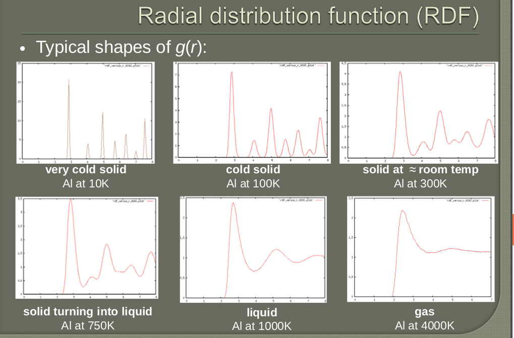
Picture stolen from Jacek Dziedzic,Gdansk University of Technology,Computational nanotechnology
